Pandas - pivot_table, Seaborn

pandas의 pivot_table 익히기

import pandas as pd
import numpy as np

df = pd.read_excel("DataScience_Ing/data/02. sales-funnel.xlsx")
df.head()

	Account	Name	Rep	Manager	Product	Quantity	Price	Status
0	714466	Trantow-Barrows	Craig Booker	Debra Henley	CPU	1	30000	presented
1	714466	Trantow-Barrows	Craig Booker	Debra Henley	Software	1	10000	presented
2	714466	Trantow-Barrows	Craig Booker	Debra Henley	Maintenance	2	5000	pending
3	737550	Fritsch, Russel and Anderson	Craig Booker	Debra Henley	CPU	1	35000	declined
4	146832	Kiehn-Spinka	Daniel Hilton	Debra Henley	CPU	2	65000	won

# index 값을 key 해서 지정이 없으면 숫자형 데이터 컬럼 모두 선택
# 중복 키는 합쳐서 평균값으로 
pd.pivot_table(df, index=['Name'])

	Account	Price	Quantity
Name
Barton LLC	740150	35000	1.000000
Fritsch, Russel and Anderson	737550	35000	1.000000
Herman LLC	141962	65000	2.000000
Jerde-Hilpert	412290	5000	2.000000
Kassulke, Ondricka and Metz	307599	7000	3.000000
Keeling LLC	688981	100000	5.000000
Kiehn-Spinka	146832	65000	2.000000
Koepp Ltd	729833	35000	2.000000
Kulas Inc	218895	25000	1.500000
Purdy-Kunde	163416	30000	1.000000
Stokes LLC	239344	7500	1.000000
Trantow-Barrows	714466	15000	1.333333

# index 여러개 지정 가능
pd.pivot_table(df,index=["Name","Rep","Manager"])

			Account	Price	Quantity
Name	Rep	Manager
Barton LLC	John Smith	Debra Henley	740150	35000	1.000000
Fritsch, Russel and Anderson	Craig Booker	Debra Henley	737550	35000	1.000000
Herman LLC	Cedric Moss	Fred Anderson	141962	65000	2.000000
Jerde-Hilpert	John Smith	Debra Henley	412290	5000	2.000000
Kassulke, Ondricka and Metz	Wendy Yule	Fred Anderson	307599	7000	3.000000
Keeling LLC	Wendy Yule	Fred Anderson	688981	100000	5.000000
Kiehn-Spinka	Daniel Hilton	Debra Henley	146832	65000	2.000000
Koepp Ltd	Wendy Yule	Fred Anderson	729833	35000	2.000000
Kulas Inc	Daniel Hilton	Debra Henley	218895	25000	1.500000
Purdy-Kunde	Cedric Moss	Fred Anderson	163416	30000	1.000000
Stokes LLC	Cedric Moss	Fred Anderson	239344	7500	1.000000
Trantow-Barrows	Craig Booker	Debra Henley	714466	15000	1.333333

pd.pivot_table(df,index=["Manager","Rep"])

		Account	Price	Quantity
Manager	Rep
Debra Henley	Craig Booker	720237.0	20000.000000	1.250000
	Daniel Hilton	194874.0	38333.333333	1.666667
	John Smith	576220.0	20000.000000	1.500000
Fred Anderson	Cedric Moss	196016.5	27500.000000	1.250000
	Wendy Yule	614061.5	44250.000000	3.000000

# 평균 낼 컬럼 지정 values=['컬럼명']
pd.pivot_table(df, index=["Manager","Rep"], values=["Price"])

		Price
Manager	Rep
Debra Henley	Craig Booker	20000.000000
	Daniel Hilton	38333.333333
	John Smith	20000.000000
Fred Anderson	Cedric Moss	27500.000000
	Wendy Yule	44250.000000

# 기본 평균 => 합계 aggfunc=np.sum
pd.pivot_table(df, index=["Manager","Rep"], values=["Price"], aggfunc=np.sum)

		Price
Manager	Rep
Debra Henley	Craig Booker	80000
	Daniel Hilton	115000
	John Smith	40000
Fred Anderson	Cedric Moss	110000
	Wendy Yule	177000

# price의 평균과 갯수
pd.pivot_table(df, index=["Manager","Rep"], values=["Price"], aggfunc=[np.mean, len])

		mean	len
		Price	Price
Manager	Rep
Debra Henley	Craig Booker	20000.000000	4
	Daniel Hilton	38333.333333	3
	John Smith	20000.000000	2
Fred Anderson	Cedric Moss	27500.000000	4
	Wendy Yule	44250.000000	4

# Product 상품을 columns로 가격 합계, 없는 건 NaN
# columns : 데이터를 컬럼명으로 바꿔줌
pd.pivot_table(df, index=['Manager', 'Rep'], values=['Price'], columns=['Product'],
               aggfunc=[np.sum])

		sum
		Price
	Product	CPU	Maintenance	Monitor	Software
Manager	Rep
Debra Henley	Craig Booker	65000.0	5000.0	NaN	10000.0
	Daniel Hilton	105000.0	NaN	NaN	10000.0
	John Smith	35000.0	5000.0	NaN	NaN
Fred Anderson	Cedric Moss	95000.0	5000.0	NaN	10000.0
	Wendy Yule	165000.0	7000.0	5000.0	NaN

# Product 상품을 columns로 가격 합계
# fill_value=입력값 : NaN 값을 입력값으로 바꿔줌
pd.pivot_table(df, index=['Manager', 'Rep'], values=['Price'], columns=['Product'],
               aggfunc=[np.sum], fill_value=0)

		sum
		Price
	Product	CPU	Maintenance	Monitor	Software
Manager	Rep
Debra Henley	Craig Booker	65000	5000	0	10000
	Daniel Hilton	105000	0	0	10000
	John Smith	35000	5000	0	0
Fred Anderson	Cedric Moss	95000	5000	0	10000
	Wendy Yule	165000	7000	5000	0

pd.pivot_table(df,index=["Manager","Rep","Product"],
               values=["Price","Quantity"],aggfunc=[np.sum],fill_value=0)

			sum
			Price	Quantity
Manager	Rep	Product
Debra Henley	Craig Booker	CPU	65000	2
		Maintenance	5000	2
		Software	10000	1
	Daniel Hilton	CPU	105000	4
		Software	10000	1
	John Smith	CPU	35000	1
		Maintenance	5000	2
Fred Anderson	Cedric Moss	CPU	95000	3
		Maintenance	5000	1
		Software	10000	1
	Wendy Yule	CPU	165000	7
		Maintenance	7000	3
		Monitor	5000	2

pd.pivot_table(df,index=["Manager","Rep","Product"],
               values=["Price","Quantity"],
               aggfunc=[np.sum,np.mean], fill_value=0)

			sum		mean
			Price	Quantity	Price	Quantity
Manager	Rep	Product
Debra Henley	Craig Booker	CPU	65000	2	32500	1.0
		Maintenance	5000	2	5000	2.0
		Software	10000	1	10000	1.0
	Daniel Hilton	CPU	105000	4	52500	2.0
		Software	10000	1	10000	1.0
	John Smith	CPU	35000	1	35000	1.0
		Maintenance	5000	2	5000	2.0
Fred Anderson	Cedric Moss	CPU	95000	3	47500	1.5
		Maintenance	5000	1	5000	1.0
		Software	10000	1	10000	1.0
	Wendy Yule	CPU	165000	7	82500	3.5
		Maintenance	7000	3	7000	3.0
		Monitor	5000	2	5000	2.0

#margins=True 합계(All)를 추가 함
pd.pivot_table(df,index=["Manager","Rep","Product"],
               values=["Price","Quantity"],
               aggfunc=[np.sum,np.mean], fill_value=0, margins=True)

			sum		mean
			Price	Quantity	Price	Quantity
Manager	Rep	Product
Debra Henley	Craig Booker	CPU	65000	2	32500.000000	1.000000
		Maintenance	5000	2	5000.000000	2.000000
		Software	10000	1	10000.000000	1.000000
	Daniel Hilton	CPU	105000	4	52500.000000	2.000000
		Software	10000	1	10000.000000	1.000000
	John Smith	CPU	35000	1	35000.000000	1.000000
		Maintenance	5000	2	5000.000000	2.000000
Fred Anderson	Cedric Moss	CPU	95000	3	47500.000000	1.500000
		Maintenance	5000	1	5000.000000	1.000000
		Software	10000	1	10000.000000	1.000000
	Wendy Yule	CPU	165000	7	82500.000000	3.500000
		Maintenance	7000	3	7000.000000	3.000000
		Monitor	5000	2	5000.000000	2.000000
All			522000	30	30705.882353	1.764706

Seaborn

• Matplotib 과 함께 사용

• 기본색감부터 이쁨

• https://seaborn.pydata.org/index.html

• https://datascienceschool.net/view-notebook/4c2d5ff1caab4b21a708cc662137bc65/

pip install seaborn

Collecting seaborn
  Downloading seaborn-0.10.1-py3-none-any.whl (215 kB)
Requirement already satisfied: numpy>=1.13.3 in c:\programdata\anaconda3\envs\r_study\lib\site-packages (from seaborn) (1.19.0)
Requirement already satisfied: pandas>=0.22.0 in c:\programdata\anaconda3\envs\r_study\lib\site-packages (from seaborn) (1.0.5)
Collecting scipy>=1.0.1
  Downloading scipy-1.5.1-cp37-cp37m-win_amd64.whl (31.2 MB)
Requirement already satisfied: matplotlib>=2.1.2 in c:\programdata\anaconda3\envs\r_study\lib\site-packages (from seaborn) (3.3.0)
Requirement already satisfied: pytz>=2017.2 in c:\programdata\anaconda3\envs\r_study\lib\site-packages (from pandas>=0.22.0->seaborn) (2020.1)
Requirement already satisfied: python-dateutil>=2.6.1 in c:\programdata\anaconda3\envs\r_study\lib\site-packages (from pandas>=0.22.0->seaborn) (2.8.1)
Requirement already satisfied: pillow>=6.2.0 in c:\programdata\anaconda3\envs\r_study\lib\site-packages (from matplotlib>=2.1.2->seaborn) (7.2.0)
Requirement already satisfied: pyparsing!=2.0.4,!=2.1.2,!=2.1.6,>=2.0.3 in c:\programdata\anaconda3\envs\r_study\lib\site-packages (from matplotlib>=2.1.2->seaborn) (2.4.7)
Requirement already satisfied: cycler>=0.10 in c:\programdata\anaconda3\envs\r_study\lib\site-packages (from matplotlib>=2.1.2->seaborn) (0.10.0)
Requirement already satisfied: kiwisolver>=1.0.1 in c:\programdata\anaconda3\envs\r_study\lib\site-packages (from matplotlib>=2.1.2->seaborn) (1.2.0)
Requirement already satisfied: six>=1.5 in c:\programdata\anaconda3\envs\r_study\lib\site-packages (from python-dateutil>=2.6.1->pandas>=0.22.0->seaborn) (1.15.0)
Installing collected packages: scipy, seaborn
Successfully installed scipy-1.5.1 seaborn-0.10.1
Note: you may need to restart the kernel to use updated packages.

import matplotlib.pyplot as plt
%matplotlib inline

import seaborn as sns

x  = np.linspace(0, 14, 100)
y1 = np.sin(x)
y2 = 2*np.sin(x+0.5)
y3 = 3*np.sin(x+1.0)
y4 = 4*np.sin(x+1.5)

plt.figure(figsize=(10, 6))
plt.plot(x,y1, x,y2, x,y3, x,y4)
plt.show()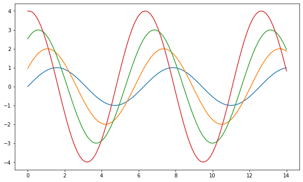

sns.set_style('white')

plt.figure(figsize=(10,6))
plt.plot(x,y1, x,y2, x,y3, x,y4)

sns.despine() # 그래프 외각선 삭제
plt.show()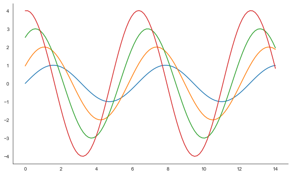

sns.set_style("dark")

plt.figure(figsize=(10,6))
plt.plot(x,y1, x,y2, x,y3, x,y4)
plt.show()

# tips 요일별 점심, 저녁, 흡연여부, 식사금액, 팁
tips = sns.load_dataset('tips')
tips.head()

	total_bill	tip	sex	smoker	day	time	size
0	16.99	1.01	Female	No	Sun	Dinner	2
1	10.34	1.66	Male	No	Sun	Dinner	3
2	21.01	3.50	Male	No	Sun	Dinner	3
3	23.68	3.31	Male	No	Sun	Dinner	2
4	24.59	3.61	Female	No	Sun	Dinner	4

sns.set_style('whitegrid')

plt.figure(figsize=(8, 6))
sns.boxplot(x=tips['total_bill'])
plt.show()

plt.figure(figsize=(8, 6))
sns.boxplot(x = 'day', y='total_bill', data = tips)
plt.show()

plt.figure(figsize=(8, 6))
sns.boxplot(x = 'day', y='total_bill', hue='smoker', data = tips, palette='Set3')
plt.show()

plt.figure(figsize=(8,6))
# swarmplot은 stripplot과 비슷하지만 데이터를 나타내는 점이 겹치지 않도록 옆으로 이동
sns.swarmplot(x="day", y="total_bill", data=tips, color=".5")
plt.show()

# boxplot과 swarmplot 합치기
plt.figure(figsize=(8,6))
sns.boxplot(x="day", y="total_bill", data=tips)
sns.swarmplot(x="day", y="total_bill", data=tips, color=".25")
plt.show()

# https://stricky.tistory.com/124
sns.set_style("darkgrid")
sns.lmplot(x="total_bill", y="tip", data=tips, size=7)
plt.show()

C:\ProgramData\Anaconda3\envs\r_study\lib\site-packages\seaborn\regression.py:573: UserWarning: The `size` parameter has been renamed to `height`; please update your code.
  warnings.warn(msg, UserWarning)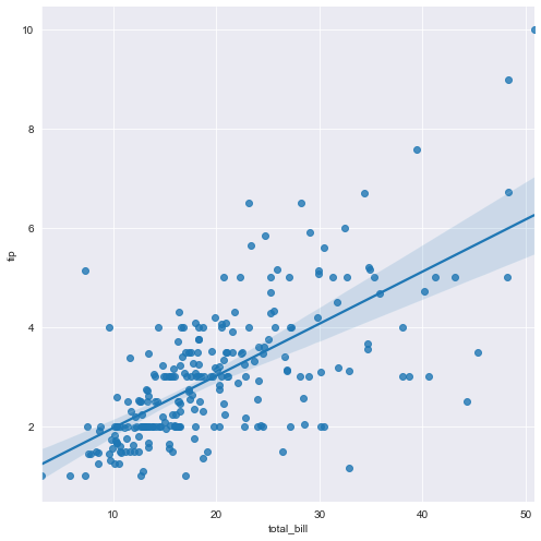

sns.lmplot(x="total_bill", y="tip", hue="smoker", data=tips, size=7)
plt.show()

C:\ProgramData\Anaconda3\envs\r_study\lib\site-packages\seaborn\regression.py:573: UserWarning: The `size` parameter has been renamed to `height`; please update your code.
  warnings.warn(msg, UserWarning)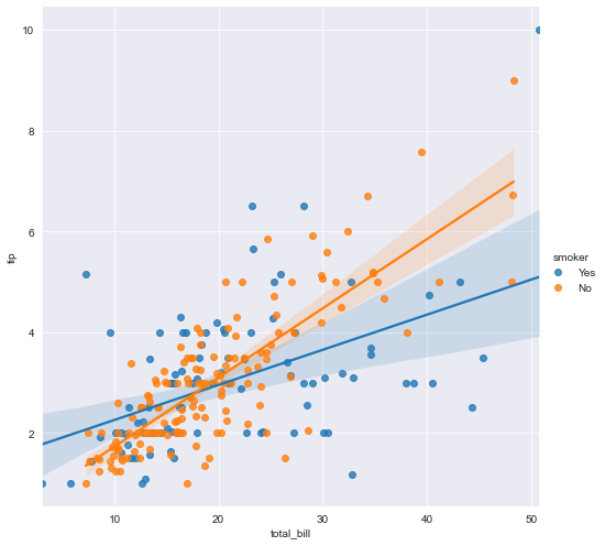

# palette : 준비된 색상 사용
sns.lmplot(x="total_bill", y="tip", hue="smoker", data=tips, palette="Set1", size=7)
plt.show()

C:\ProgramData\Anaconda3\envs\r_study\lib\site-packages\seaborn\regression.py:573: UserWarning: The `size` parameter has been renamed to `height`; please update your code.
  warnings.warn(msg, UserWarning)

uniform_data = np.random.rand(10, 12)
uniform_data

array([[0.78267668, 0.05329411, 0.30891095, 0.88363145, 0.70073013,
        0.82364346, 0.93755569, 0.88168907, 0.0611389 , 0.95009859,
        0.90326253, 0.44996643],
       [0.41058408, 0.99793684, 0.98629444, 0.56033547, 0.22137451,
        0.20827601, 0.67043358, 0.65044688, 0.88602835, 0.07627844,
        0.73710037, 0.2888487 ],
       [0.95512591, 0.08189851, 0.98961883, 0.4498224 , 0.18747087,
        0.07756019, 0.10771306, 0.06518051, 0.13345012, 0.08949381,
        0.23818968, 0.17667309],
       [0.0054546 , 0.93265432, 0.89488956, 0.29465216, 0.26264216,
        0.21948854, 0.25496933, 0.48549471, 0.53208498, 0.09197529,
        0.68160834, 0.13727799],
       [0.21337441, 0.39321309, 0.26175172, 0.64866811, 0.35011416,
        0.30610248, 0.13096216, 0.44142762, 0.65704918, 0.35620841,
        0.43864634, 0.69212818],
       [0.69440397, 0.43158162, 0.05624385, 0.66550322, 0.56875231,
        0.74785321, 0.86025044, 0.80489812, 0.32656482, 0.25604858,
        0.62767696, 0.24667137],
       [0.59842438, 0.06233472, 0.50291815, 0.43099899, 0.15199756,
        0.51611582, 0.76908056, 0.13003266, 0.16484196, 0.18200507,
        0.91531206, 0.4690069 ],
       [0.86777144, 0.45906632, 0.35278867, 0.4299843 , 0.65543608,
        0.01189033, 0.59340044, 0.2619662 , 0.42551808, 0.2914703 ,
        0.07028432, 0.44401921],
       [0.99550615, 0.26756271, 0.73404515, 0.17040982, 0.43780665,
        0.19886461, 0.6734527 , 0.55325288, 0.05469495, 0.87586727,
        0.56640452, 0.65712259],
       [0.09218315, 0.99514556, 0.53144343, 0.61129401, 0.71577029,
        0.19014461, 0.09339864, 0.33209108, 0.75898979, 0.18667022,
        0.03908457, 0.90274583]])

# heatmap : https://rfriend.tistory.com/419
# seaborn은 데이터가 2차원 피벗 테이블 형태의 DataFrame으로 집계가 되어 있으면 
# sns.heatmap() 함수로 매우 간단하게 히트맵을 그려줍니다. 
sns.heatmap(uniform_data)
plt.show()

sns.heatmap(uniform_data, vmin=0, vmax=1) # vimn, vmax 색상 막대 범위
plt.show()

# 연도별 월별 항공기 승객수
flights = sns.load_dataset("flights")
flights.head(5)

	year	month	passengers
0	1949	January	112
1	1949	February	118
2	1949	March	132
3	1949	April	129
4	1949	May	121

# pivot 기능으로 간편하게 월별, 연도별로 구분할 수 있다. 
flights = flights.pivot('month', 'year', 'passengers')
flights.head()

year	1949	1950	1951	1952	1953	1954	1955	1956	1957	1958	1959	1960
month
January	112	115	145	171	196	204	242	284	315	340	360	417
February	118	126	150	180	196	188	233	277	301	318	342	391
March	132	141	178	193	236	235	267	317	356	362	406	419
April	129	135	163	181	235	227	269	313	348	348	396	461
May	121	125	172	183	229	234	270	318	355	363	420	472

plt.figure(figsize=(10, 8))
sns.heatmap(flights)
plt.show()

plt.figure(figsize=(10,8))
# annot=True 일때 자리수 지정 ex) fmt='.2f' 소수점 2자리 
sns.heatmap(flights, annot=True, fmt="d") 
plt.show()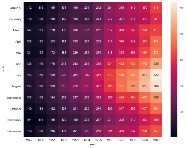

sns.set(style="ticks") # ticks : grid 제거
# iris 머신러닝에서 기본적으로 사용한 아이리스 꽃 관련 데이터
# 꽃잎, 꽃받침의 너비와 폭을 가지고 종(species)을 구분 하기 위한 데이터
iris = sns.load_dataset("iris")
iris.head(10)

	sepal_length	sepal_width	petal_length	petal_width	species
0	5.1	3.5	1.4	0.2	setosa
1	4.9	3.0	1.4	0.2	setosa
2	4.7	3.2	1.3	0.2	setosa
3	4.6	3.1	1.5	0.2	setosa
4	5.0	3.6	1.4	0.2	setosa
5	5.4	3.9	1.7	0.4	setosa
6	4.6	3.4	1.4	0.3	setosa
7	5.0	3.4	1.5	0.2	setosa
8	4.4	2.9	1.4	0.2	setosa
9	4.9	3.1	1.5	0.1	setosa

sns.pairplot(iris)
plt.show()

sns.pairplot(iris, hue="species")
plt.show()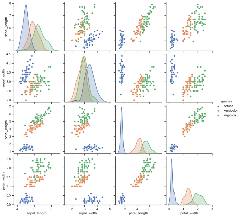

sns.pairplot(iris, vars=["sepal_width", "sepal_length"])
plt.show()

sns.pairplot(iris, x_vars=["sepal_width", "sepal_length"], 
             y_vars=["petal_width", "petal_length"])
plt.show()

Pandas2.html

1.19MB